この章では、アンサンブルカルマンフィルタについて述べる。
カルマンフィルタ
Section 1.6
\[
\mathbf{x}^\mathrm{a} = \mathbf{x}^\mathrm{b} + \mathbf{K}(\mathbf{y}^\mathrm{o} - \mathbf{Hx}^\mathrm{b})
\] と書くことができる。 ここで
\[
\mathbf{K} = \mathbf{BH}^\mathrm{T}(\mathbf{HBH}^\mathrm{T} + \mathbf{R})^{-1}
\tag{4.1}\]
はカルマンゲインである。
カルマンゲインを用いると、解析誤差共分散 Section 1.6
\[
\mathbf{P}_\mathrm{a} = (\mathbf{I} - \mathbf{KH})\mathbf{B}(\mathbf{I} - \mathbf{KH})^\mathrm{T} + \mathbf{KRK}^\mathrm{T} = (\mathbf{I} - \mathbf{KH})\mathbf{B}
\tag{4.2}\]
となり、背景誤差共分散よりも縮小する。
アンサンブルカルマンフィルタ
アンサンブルカルマンフィルタ(EnKF: Ensemble Kalman Filter Evensen (1994 ) )では背景誤差共分散\(\mathbf{B}\) をモデル予報のアンサンブルからの標本共分散\(\mathbf{P}_\mathrm{b}\) で近似する。
\[
\begin{aligned}
\bar{\mathbf{x}}^\mathrm{b} &= \frac{1}{k}\sum_{i=1}^k \mathbf{x}^\mathrm{b}_i\\
\mathbf{P}^\mathrm{b} &= \frac{1}{k-1}\sum_{i=1}^k(\mathbf{x}^\mathrm{b}_i-\bar{\mathbf{x}}^\mathrm{b})(\mathbf{x}^\mathrm{b}_i-\bar{\mathbf{x}}^\mathrm{b})^\mathrm{T}
\end{aligned}
\tag{4.3}\]
同様に解析値の平均と誤差共分散は次の式で定義される。
\[
\begin{aligned}
\bar{\mathbf{x}}^\mathrm{a} &= \frac{1}{k}\sum_{i=1}^k \mathbf{x}^\mathrm{a}_i\\
\mathbf{P}_\mathrm{a} &= \frac{1}{k-1}\sum_{i=1}^k(\mathbf{x}^\mathrm{a}_i-\bar{\mathbf{x}}^\mathrm{a})(\mathbf{x}^\mathrm{a}_i-\bar{\mathbf{x}}^\mathrm{a})^\mathrm{T}\\
\end{aligned}
\tag{4.4}\]
EnKFの更新式は次のように書ける。 \[
\begin{aligned}
\bar{\mathbf{x}}^\mathrm{a} &= \bar{\mathbf{x}}^\mathrm{b} + \mathbf{K}(\bar{\mathbf{y}}^\mathrm{o} - \mathbf{H}\bar{\mathbf{x}}^\mathrm{b})\\
\mathbf{x}^\mathrm{'a} &= \mathbf{x}^\mathrm{'b} + \tilde{\mathbf{K}}(\mathbf{y}^{'\mathrm{o}} - \mathbf{H}\mathbf{x}^\mathrm{'b})\\
\end{aligned}
\tag{4.5}\]
ここで、\(\mathbf{y}^{'\mathrm{o}}\) は観測誤差の確率密度分布からランダムに選んだ摂動、\(\tilde{\mathbf{K}}\) は偏差の更新に用いるカルマンゲインである。 EnKFでは\(\tilde{\mathbf{K}} = \mathbf{K}\) を用い、\((\mathbf{y}^{'\mathrm{o}}\) は観測誤差の確率密度分布からランダムに抽出する。 これを摂動観測法 (PO: Perturbed Observations, Burgers et al. 1998 ; Houtekamer and Mitchell 1998 ) と呼ぶ (Section 4.5
全てのアンサンブルメンバーが同じ観測を同化すると\(\mathbf{y}^{'\mathrm{o}} = 0\) となるので解析誤差共分散は Equation 4.5 より \[
\mathbf{P}_\mathrm{a} = (\mathbf{I} - \mathbf{KH})\mathbf{P}_\mathrm{b}(\mathbf{I} - \mathbf{KH})^\mathrm{T}\
\tag{4.6}\]
Equation 4.2 と比較すると Equation 4.6 は、\(\mathbf{KRK}^\mathrm{T}\) の項がなく、\(\mathbf{I} - \mathbf{KH}\) 倍、解析誤差共分散が過小評価されている。
観測誤差が\(\mathbf{y}^{'\mathrm{o}}\ne 0\) の場合,解析誤差共分散は次のようになる。
\[
\begin{aligned}
\mathbf{P}_\mathrm{a} &= (\mathbf{I} - \mathbf{KH})\mathbf{P}_\mathrm{b}(\mathbf{I} - \mathbf{KH})^\mathrm{T}\\
&+\mathbf{K}\left(\overline{\mathbf{y}'\mathbf{y}^{'\mathrm{T}}}
-\overline{\mathbf{Hx}^{'\mathrm{b}}\mathbf{y}^{'\mathrm{T}}}
-\overline{\mathbf{y}'\mathbf{x}^{'\mathrm{bT}}\mathbf{H}^\mathrm{T}}
\right)\mathbf{K}^\mathrm{T}\\
&+\overline{\mathbf{x}^{'\mathrm{b}}\mathbf{y}^{'\mathrm{T}}}\mathbf{K}^\mathrm{T} + \mathbf{K}\overline{\mathbf{y}'\mathbf{x}^{'\mathrm{bT}}}
\end{aligned}
\tag{4.7}\]
観測ノイズが\(\mathbf{R} = E\left(\overline{\mathbf{y}'\mathbf{y}^{'\mathrm{T}}}\right)\) で与えられ,\(E\left(\overline{\mathbf{x}^{'\mathrm{b}}\mathbf{y}^{'\mathrm{T}}}\right) = 0\) ならば\(\mathbf{P}_\mathrm{a}\) の期待値は Equation 4.2 と等しくなる。
解析誤差共分散推定に対する標本誤差の影響
有限のアンサンブル数では,背景誤差共分散の推定において標本誤差が生じる。 観測誤差に摂動を与えると,観測誤差共分散にも標本誤差が含まれる。 これらの誤差が解析誤差共分散にどのように影響を与えるか簡単な実験で示す(Whitaker and Hamill 2002 ) 。 摂動観測法ありとなし(解析誤差共分散を Equation 4.2 で計算)とを比較する。
状態ベクトル\(\mathbf{x}^\mathrm{b}\) 及び観測\(\mathbf{y}\)
\(\mathbf{x}^\mathrm{b}\) と\(\mathbf{y}\) とは同じ量つまり\(\mathbf{H}=1\) 試行回数1,000,000回
アンサンブルメンバー数5
\(\mathbf{x}^\mathrm{b}\) 正規分布\(N(0, 1)\) からランダムに選ぶ。背景誤差分散は自由度4の\(\chi^2\) 分布で平均は1
観測誤差分散1のEnKFでは観測を\(N(0, 1)\) から選択し平均0分散1となるように調整する。
Code
<- 1000000 <- 5 <- m - 1 <- 1 set.seed (514 )<- scale (matrix (rnorm (m * n), nrow = m), scale = FALSE ) <- scale (matrix (rnorm (m * n), nrow = m), scale = FALSE )<- colMeans (Xb^ 2 ) * m / dof<- Pb / (Pb + R)<- (1 - K) * Pb<- colMeans (Xb * y) * m / dof<- (1 - K)^ 2 * Pb<- K^ 2 * R<- 2 * K * yx * (1 - K)<- zeta1 + zeta2 + zeta3
Code
palette ("Tableau 10" )<- seq (0 , 2 , length.out= 101 )<- p * dofplot (p, dchisq (var, dof) / sum (dchisq (var, dof)), type = "l" , lwd = 2 , col = "black" ,xlab = "variance" , ylab = "relative frequency" , ylim = c (0 , 0.05 ))abline (v = 0.5 , lty = "solid" , col = "black" )<- hist (Pa, breaks = seq (0 , 2 , length= 101 ), plot = F, right = FALSE )lines (stepfun (h$ breaks, c (NA , h$ counts / sum (h$ counts), NA ), f = 0 ),do.points = FALSE , col = 1 )abline (v = mean (Pa), lty = "dotted" , col = 1 )<- Pa_PO >= 0 & Pa_PO <= 2 <- hist (Pa_PO[within_bins], breaks = seq (0 , 2 , length= 101 ), plot = F, right = FALSE )lines (stepfun (h$ breaks, c (NA , h$ counts / sum (h$ counts), NA ), f = 0 ),do.points = FALSE , col = 2 )abline (v = mean (Pa_PO), lty = "dashed" , col = 2 )legend ("topright" , c ("Pb" , "Pa" , "Pa PO" ), col = c ("black" , 1 , 2 ), lwd = 2 )palette ("R4" )
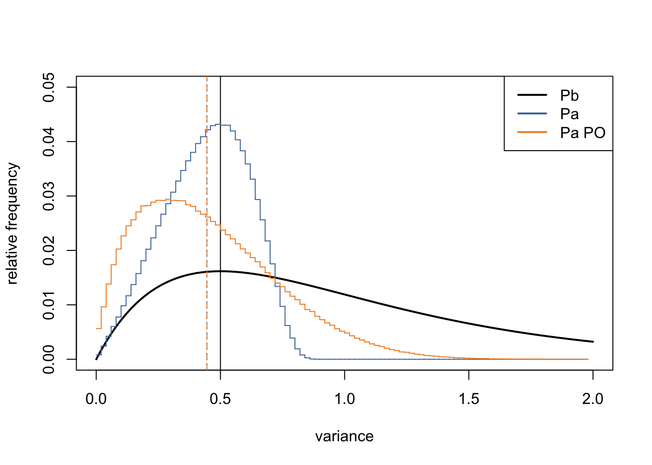
背景誤差共分散(Figure 4.1 黒)は\(\chi^2\) 分布に従う。 観測を同化すると,小さい値の振幅が大きくなり分散は小さくなる(青)。 摂動観測法の解析誤差分散(橙)は小さい値の確率が高い。
Equation 4.1 と Equation 4.2 より解析誤差共分散は背景誤差共分散に非線型に依存することが分かる。 \[
\mathbf{P}_\mathrm{a} = (1 - \mathbf{K})\mathbf{P}_\mathrm{b} = \left(1 - \frac{\mathbf{P}_\mathrm{b}}{\mathbf{P}_\mathrm{b} + \mathbf{R}}\right)\mathbf{P}_\mathrm{b}
\] 観測に対する摂動の有無は関係なく、標本誤差のため\(\mathbf{P}^\mathrm{b}\) は確率変数であるため,\(\mathbf{P}^\mathrm{a}\) も確率変数である。 \(\mathbf{P}_\mathrm{b}=1\) に対する\(\mathbf{P}_\mathrm{a}\) の期待値は0.5であるが,\(\mathbf{P}_\mathrm{a}\) の平均は約0.44である。 \(\mathbf{P}_\mathrm{b}\) にバイアスがなくても、\(\mathbf{P}_\mathrm{a}\) にバイアスが生じるのは同系交配(inbreeding)の影響である(Houtekamer and Mitchell 1998 ) 。
非線型性に起因す誤差分散の過小バイアスは、アンサンブル数を増やすと減少する。 \(\mathbf{P}^\mathrm{b}\) が平均の周りに狭く対称に分布し,カルマンゲインで非線型変換された\(\mathbf{P}^\mathrm{a}\) も対称に近づくためである。
観測摂動法EnKFに対しては,Equation 4.7 で与えられる解析誤差分散\(\mathbf{P}^\mathrm{a}_{\mathrm{PO}}\) は,この実験において以下のように簡単になる。 \[
\mathbf{P}^\mathrm{a}_{\mathrm{PO}} = \underbrace{(1 - \mathbf{K})^2\mathbf{P}^\mathrm{b}}_{\zeta_1} + \underbrace{\mathbf{K}^2\mathbf{R}}_{\zeta_2} + \underbrace{2\mathbf{K}\overline{\mathbf{y}'\mathbf{x}^{'\mathrm{b}}}(1 - \mathbf{K})}_{\zeta_3}
\]
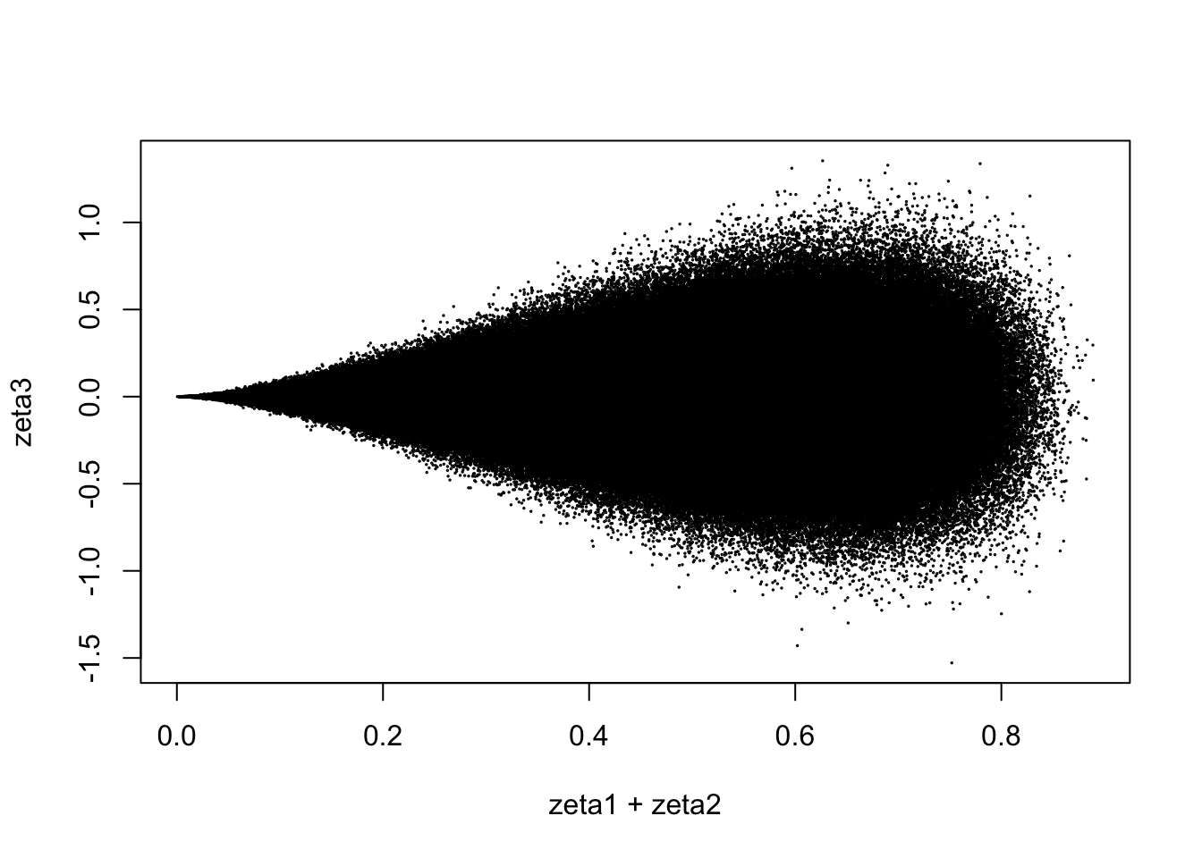
\(\mathbf{P}^\mathrm{a}_{\mathrm{PO}}\) の平均は\(\mathbf{P}^\mathrm{a}\) と同じになるが、標本誤差の影響で分布は幅広く,誤差は大きくなる。
Code
plot (zeta1 + zeta2, zeta3, cex = 0.1 )
\(\zeta_1 + \zeta_2\) が大きくなると\(\zeta_3\) の分散が大きくなる。 ノイズ\(\zeta_3\) は\(\zeta_1+\zeta_2\) が大きくなるほど分布を両側に広げるために,\(\mathbf{P}^\mathrm{a}_{\mathrm{PO}}\) の分布が左に歪む。
単一観測の同化
個々の観測が独立であれば、\(\mathbf{R}\) は対角で、一要素ずつ順番に同化しても結果は変わらない(Anderson 2003 ) 。 これを利用して、演算を簡略化し、同化を2段階で行う。
単一の測定値をアンサンブル予報から推定した観測変数に同化し、インクリメント(変化量)\(\Delta y_i\) を求める。ここで\(i\) はアンサンブルの番号\(i=1, \dots N\) 。
各状態変数の各アンサンブル標本について、対応するインクリメントを線型回帰で求める。 状態変数及び観測変数との間に、先験関係がガウス分布であることを仮定し、最小二乗法で直線を当てはめている。 非線型であることも考えられる観測演算子に対して、線型化を施し逆函数を求めていることに相当する。
\(y\) の変化に対する\(x\) の変化の回帰は次のように書ける。 \[
\Delta x = \frac{ \mathrm{cov}(x, y)}{\mathrm{var}(y)}\Delta y
\tag{4.8}\]
長さ\(n\) の状態ベクトル\(\mathbf{x}\) 及び、それから求めた長さ\(m\) の観測相当量\(\mathbf{y}=h(\mathbf{x})\) を結合した長さ\(k+m\) のベクトル \[
\mathbf{z} = \begin{bmatrix}\mathbf{x}\\h(\mathbf{x})\end{bmatrix}
\]
を考える。 これを結合状態・観測空間とよぶ。 その共分散は
\[
\boldsymbol\Sigma_\mathrm{a} = [\boldsymbol\Sigma_\mathrm{f}^{-1} + \mathbf{H}^\mathrm{T}\mathbf{R}^{-1}\mathbf{H}]^{-1}
\tag{4.9}\]
アンサンブル平均は \[
\bar{\mathbf{z}}^\mathrm{a} = \boldsymbol\Sigma_\mathrm{a}[\boldsymbol\Sigma_\mathrm{f}^{-1}\bar{\mathbf{z}}^\mathrm{f} + \mathbf{H}^\mathrm{T}\mathbf{R}^{-1}\mathbf{y}^\mathrm{o}]
\tag{4.10}\]
1個のスカラー観測に対しては、\(\boldsymbol\Sigma_\mathrm{f},\,\boldsymbol\Sigma_\mathrm{a}\) の左上から\(n\times n\) の部分は、それぞれ\(\mathbf{P}_\mathrm{f},\,\mathbf{P}_\mathrm{a}\) であり、\(k\) 列目は変数間の共分散\(\mathbf{s}^\mathrm{f},\,\mathbf{s}^\mathrm{a}\) 、\(\mathbf{s}^\mathrm{f}_k=s^\mathrm{f},\,\mathbf{s}^\mathrm{a}_k=s^\mathrm{a}\) は\(\mathbf{y}^\mathrm{f}=h(\mathbf{x}^\mathrm{f}),\,\mathbf{y}^\mathrm{a}=h(\mathbf{x}^\mathrm{a})\) の分散を表す。 線型演算子\(\mathbf{H}=\begin{bmatrix}0&0&\dots&1\end{bmatrix}\) は最後の要素\(y\) を取り出す\(1\times k\) の行列である。 観測誤差共分散行列\(\mathbf{R}\) はスカラーの分散\(r\) で表される。
式(Equation 4.9 ), (Equation 4.10 )はそれぞれ、
\[
\boldsymbol\Sigma_\mathrm{a} = \left(\mathbf{I} - \frac{1}{r + s^\mathrm{f}}\boldsymbol\Sigma^{0k}_\mathrm{f}\right)\boldsymbol\Sigma_\mathrm{f},
\tag{4.11}\]
\[
\Delta\bar{\mathbf{z}} = \mathbf{z}^\mathrm{a} - \mathbf{z}^\mathrm{f} = \frac{y^\mathrm{o}-\bar{y}^\mathrm{f}}{r + s^\mathrm{f}}\mathbf{s}^\mathrm{f}
\tag{4.12}\]
と簡単になる。ここで
\[
\boldsymbol\Sigma^{0k}_\mathrm{f} = \boldsymbol\Sigma_\mathrm{f}\mathbf{H}^\mathrm{T}\mathbf{H}
\] は、\(\boldsymbol\Sigma_\mathrm{f}\) の1から\(n\) 列目を0とし、\(k\) 列目だけを残した行列である。 観測変数の分散は
\[
s^\mathrm{a} = \frac{1}{1/s^\mathrm{f} + 1/r} = \frac{s^\mathrm{f}r}{s^\mathrm{f} + r}
\tag{4.13}\]
解析値は
\[
\bar{y}^\mathrm{a} = s^\mathrm{a}(\bar{y}^\mathrm{f}/s^\mathrm{f} + y^\mathrm{o}/r) = \frac{1}{s^\mathrm{f} +r}(r\bar{y}^\mathrm{f} + s^\mathrm{f}y^\mathrm{o})
\tag{4.14}\]
観測変数のインクリメントは
\[
\Delta\bar{y}=\bar{y}^\mathrm{a} - \bar{y}^\mathrm{f} =\frac{s^\mathrm{f}}{s^\mathrm{f} + r}(y^\mathrm{o} - \bar{y}^\mathrm{f})
\tag{4.15}\]
となる。 一方、状態変数は
\[
\Delta\bar{x} = \bar{x}^\mathrm{a} - \bar{x}^\mathrm{f} = \frac{[s^\mathrm{f}_1, \dots, s^\mathrm{f}_n]^\mathrm{T}}{s^\mathrm{f} + r}(y^\mathrm{o} - \bar{y}^\mathrm{f}) = \frac{[s^\mathrm{f}_1, \dots, s^\mathrm{f}_n]^\mathrm{T}}{s^\mathrm{f} + r}\Delta\bar{y}
\tag{4.16}\]
となる。 これは、それぞれの状態変数に対する線型回帰(Equation 4.8 )に他ならない。
摂動法
確率的(stochastic)もしくはモンテルカルロ法に基づくアンサンブルカルマンフィルタ(Evensen 1994 ; Houtekamer and Mitchell 1998 ; Burgers et al. 1998 ) では、観測に摂動を加えるため摂動法(PO: perturbed observation)と呼ばれている。 Vetra-Carvalho et al. (2018 ) は、観測\(y^\mathrm{o}\) には測定誤差があり、それに伴う確率分布を持っているので、予測の観測推定量\(\mathbf{y}\) に摂動を加えると解釈する方が適切であるとしているが、ここでは前者に従い、平均と分散が\(y^\mathrm{o},\,r\) となる正規分布で誤差を与える。
\[
\mathbf{y}^\mathrm{o} \sim N(y^\mathrm{o}, r)
\]
各メンバーに対して線型回帰(Equation 4.16 )を適用して解析値を求める。
アンサンブル平方根フィルタ
観測に摂動を与えることに伴う標本誤差(Whitaker and Hamill 2002 ) を回避するアンサンブル平方根フィルタ(EnSRF: ensemble square-root filter)が複数考案された(Anderson 2001 ; Bishop et al. 2001 ; Whitaker and Hamill 2002 ; Tippett et al. 2003 ) 。 ここでは、スカラー観測を逐次に同化するアンサンブル調節カルマンフィルタ(EAKF: ensemble adjustment filter, Anderson 2003 ) について述べる。
アンサンブル平均からの偏差を\(\delta\) で表す。 観測変数の予報分散は\(s^\mathrm{f}\) 、解析分散は(Equation 4.13 )なので、その比 \[
\alpha = \sqrt{\frac{r}{r + s^\mathrm{f}}}
\tag{4.17}\] \(i\) の解析インクリメントは \[
\delta \mathbf{y}_i = \delta \mathbf{y}_i^\mathrm{a} -\delta \mathbf{y}_i^\mathrm{f} = (\alpha - 1) \delta \mathbf{y}_i^\mathrm{f}
\tag{4.18}\] \[
\Delta \mathbf{z}_{i} = \frac{\mathbf{s}^\mathrm{f}}{s^\mathrm{f}}\Delta \mathbf{y}_i = \frac{\mathbf{s}^\mathrm{f}}{s^\mathrm{f}}(\alpha - 1)\delta \mathbf{y}^\mathrm{f}_i
\tag{4.19}\] Equation 4.12 )を加えてアンサンブルを更新する。 \[
\mathbf{z}^\mathrm{a}_i = \mathbf{z}^\mathrm{f}_i + \frac{\mathbf{s}^\mathrm{f}}{r + s^\mathrm{f}}(y^\mathrm{o} - \bar{y}^\mathrm{f}) + \frac{\mathbf{s}^\mathrm{f}}{s^\mathrm{f}}(\alpha - 1)(\mathbf{y}^\mathrm{f}_i - \bar{y}^\mathrm{f})
\tag{4.20}\]
決定論的アンサンブルカルマンフィルタ
通常、背景場に対する修正が微小である。 このことに着目し平方根フィルタを線型近似したものが、決定論的アンサンブルカルマンフィルタ(DEnKF: deterministic EnKF, Sakov and Oke 2008 ) である。
\(\mathbf{KH}\) が小さいとき、アンサンブルカルマンフィルタの解析誤差共分散 Equation 4.6 は次のように書ける。
\[
\mathbf{P}_\mathrm{a} = \mathbf{P}_\mathrm{b} - 2\mathbf{KHP}_\mathrm{b} + \mathbf{KHP}_\mathrm{b}\mathbf{H}^\mathrm{T}\mathbf{K}^\mathrm{T} \approx (\mathbf{I} - 2\mathbf{KH})\mathbf{P}_\mathrm{b}
\tag{4.21}\]
ここで
\[
\mathbf{P}_\mathrm{b}\mathbf{H}^\mathrm{T}\mathbf{K}^\mathrm{T} = \mathbf{P}_\mathrm{b}\mathbf{H}^\mathrm{T}(\mathbf{H}\mathbf{P}_\mathrm{b}\mathbf{H}^\mathrm{T} + \mathbf{R})^{-1}\mathbf{H}\mathbf{P}_\mathrm{b} = \mathbf{K}\mathbf{H}\mathbf{P}_\mathrm{b}
\]
を用いた。
Equation 4.21 は、カルマンゲインを半分にすると理想的な解析誤差共分散 Equation 4.2 に近づくことを示唆している。
アンサンブル偏差を
\[
\delta \mathbf{x}_i = \mathbf{x}_i - \bar{\mathbf{x}}
\tag{4.22}\]
DEnKFの計算手順は次のとおりである。
与えらたアンサンブル予測に対して、Equation 4.3 の最初の式を用いて、アンサンブル平均\(\bar{\mathbf{x}}_\mathrm{b}\) とアンサンブル偏差\(\delta\mathbf{x}^\mathrm{b}\) Equation 4.22 を計算する。
Equation 4.5 の最初の式でアンサンブル平均に対して\(\bar{\mathbf{x}}^\mathrm{a}\) を解析値を求める。解析のアンサンブル偏差は、Equation 4.5 の二番目の式で\(\tilde{\mathbf{K}} = \mathbf{K}/2\) として計算する。 \[
\delta{\mathbf{x}}^\mathrm{a} = \delta{\mathbf{x}}^\mathrm{b} - \frac{1}{2}\mathbf{KH}\delta{\mathbf{x}}^\mathrm{b}
\tag{4.23}\]
アンサンブル偏差に解析値を加えて、アンサンブルの解析値 \(\mathbf{x}^\mathrm{a}_i = \delta\mathbf{x}^\mathrm{a}_i + \bar{\mathbf{x}}_\mathrm{a}\) を計算する。
この手法では、半分のカルマンゲインを用いたカルマンフィルタの解析方程式を各アンサンブルメンバに適用し、アンサンブル平均に対する解析を加えている。 EnSRF同様に摂動観測を用いていないので、決定論的フィルタである。
Equation 4.23 は、EnSRFのアンサンブル偏差の線型近似となっている。 Equation 4.23 を用いて解析誤差共分散を求めると
\[
\mathbf{P}_\mathrm{a} = (\mathbf{I} - \mathbf{KH})\mathbf{P}_\mathrm{b} + \frac{1}{4}\mathbf{KHP}_\mathrm{b}\mathbf{H}^\mathrm{T}\mathbf{K}^\mathrm{T}
\tag{4.24}\]
となる。 \(\mathbf{KH}\) が小さいとき、理想的な解析誤差共分散Equation 4.2 の良い近似となっている。 \(\mathbf{KH}\) が大きいときは、解析誤差共分散が Equation 4.24 の右辺第2項の分だけ大きくなるので、適応インフレーションとして作用する。
Equation 4.23 は \[
\delta{\mathbf{x}}^\mathrm{a} = \frac{1}{2}\delta{\mathbf{x}}^\mathrm{b} + \frac{1}{2}(\delta{\mathbf{x}}^\mathrm{b} - \mathbf{KH}\delta{\mathbf{x}}^\mathrm{b})
\tag{4.25}\]
と表すことができる。 Equation 4.25 の右辺右辺第1、2項は、それぞれアンサンブル偏差の背景値(先験値)、解析値なので、両者の平均をとっている。 すなわち、DEnKFは重み \(1/2\) の先験偏差への緩和 (RTPP: relaxation-to-prior-perturbation Zhang et al. 2004 ) に相当する (Bowler et al. 2013 ) 。
準地衡流モデル
Sakov and Oke (2008 ) を追試した 榎本 and 中下 (2022 ) の概要を紹介する。
2次元準地衡流(quasi-geostrophic, QG)方程式は中緯度における大気や海洋の大規模な流れの特徴を表すことができるため、計算量を抑えつつトイモデルよりも現実的なデータ同化の問題を検討することができる。
ここでは中緯度海洋における表層流を模した流れに対するデータ実験を行う。
QG方程式は次の式で表される。
\[
\frac{\partial q}{\partial t} = -\frac{\partial\psi}{\partial x} - \varepsilon J(\psi, q) - A\Delta^3\psi + \nabla\times\tau
\tag{4.26}\]
\(t, x, y\) ははそれぞれ時刻と東西及び南北座標,\(\psi\) は流線函数,\(J(p, q)\) はヤコビアン,\(\Delta=\partial^2/\partial x^2 + \partial^2/\partial y^2\) はラプラシアンを表す。
渦位と流線函数は
\[
q=\Delta\psi - F\psi
\tag{4.27}\]
で関係付けられる。
理想的な風応力\(\tau = -\cos(2\pi y)\) を考えると、そのカールは
\[
\nabla\times\tau = - 2\pi\sin(2\pi y)
\tag{4.28}\]
となる。
モデルの設定と計算手法の概要は次通りである。 正方形領域\(0\le x\le 1\) , \(0 \le y \le 1\) を\(129\times 129\) 点に離散化し、 境界条件は\(\psi=\Delta\psi=\Delta^2\psi=0\) とする。 内部領域のみ4次のRunge-Kutta法を用いて、時間ステップ\(\Delta t = 1.25\) で時間発展させる。 Equation 4.27 の右辺第1項は、惑星渦度を表し中央差分を用いる。 右辺第2項は、(Arakawa 1966 ) ヤコビアンを用いて非線型不安定を抑制する。 ポワッソン方程式Equation 4.27 は多重格子法を用いて解く。 標準パラメタは\(\varepsilon = 10^{-5}, A = 2\times 10^{-12}, F = 1600\) とする。
データ同化実験の一例を示す。 長期積分から25メンバをランダムに選択して、アンサンブル予報の初期値とした。 観測は真値に分散\(\sigma^2 = 4.0\) ガウス型のランダム誤差を付加した\(\psi\) とし、4ステップ毎に\(m = 300\) 個を同化した。 観測網は海面高度計を模したものとする。
サンプル数不足による偽相関を抑制するため、共分散行列に局所化を適用する。 DEnKFの特徴はETKF等とは異なり、予報共分散行列に対してSchur積(要素毎の積)による局所化が容易に行えることである。 局所化函数は、局所化半径\(r_0 = 15\) 格子のガウス型とする。 共分散膨張係数は\(\alpha = 1.06\) とする。
実験の結果を以下に示す。 境界の渦やその周辺から観測により誤差が減少し観測誤差を下回るが、渦の活動が活発な西側の南北の中央付近では最終時刻でも観測誤差程度の誤差が残る。 予報誤差標準偏差の大きな領域ではインクリメントが入りやすいことも分かる。
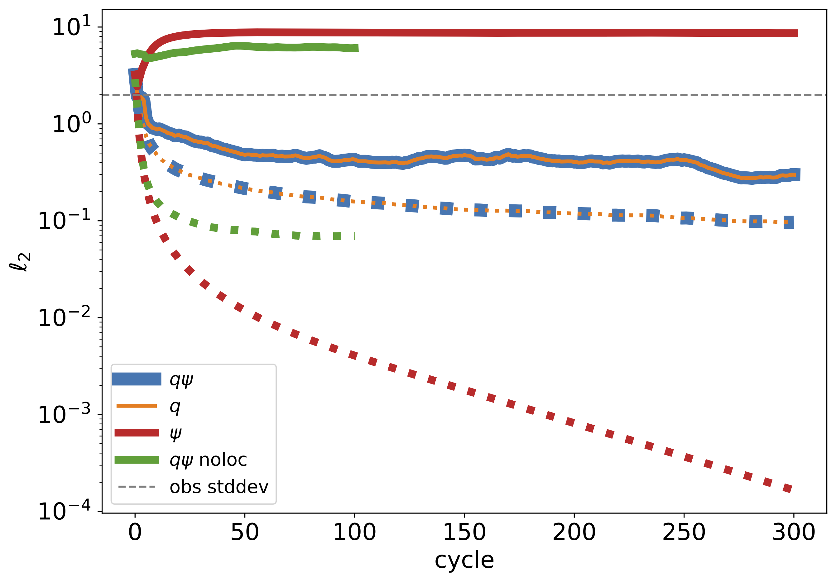
領域平均では、データ同化の初期に解析誤差は急減して観測誤差を下回る。 解析標準偏差は解析誤差を下回っており、予報誤差共分散を過小評価が示唆される。 渦位と流線函数を予報した場合も、渦位のみを予報した場合も同一の結果であり、多重格子法により流線函数が精度良く推定できている。 流線函数のみ予報し、渦位を流線函数から診断すると、渦の振幅が小さくなり適切に同化ができなかった。 局所化を用いない場合は、フィルタは発散する。
Anderson, J. L., 2001: An ensemble adjustment
Kalman filter for data assimilation.
Mon. Wea. Rev. ,
129 , 2884–2903,
https://doi.org/10.1175/1520-0493(2001)129<2884:AEAKFF>2.0.CO;2 .
——, 2003: A local least squares framework for ensemble filtering.
Mon. Wea. Rev. ,
131 , 634–642,
https://doi.org/10.1175/1520-0493(2003)131<0634:ALLSFF>2.0.CO;2 .
Arakawa, A., 1966: Computational design for long-term numerical integration of the equations of fluid motion: Two-dimensional incompressible flow Part I . J. Comput. Phys. , 1 , 119–143.
Bishop, C. H., J. Etherton, and S. J. Majumdar, 2001: Adaptive sampling with the ensemble transform
Kalman filter.
Part I : Theoretical aspects.
Mon. Wea. Rev. ,
129 , 420–436,
https://doi.org/10.1175/1520-0493(2001)129<0420:ASWTET>2.0.CO;2 .
Bowler, N. E., J. Flowerdew, and S. R. Pring, 2013: Tests of different flavours of
EnKF on a simple model.
Quart. J. Roy. Meteor. Soc. ,
139 , 1505–1519,
https://doi.org/10.1002/qj.2055 .
Burgers, G., P. J. van Leeuwen, and G. Evensen, 1998: Analysis scheme in the ensemble
Kalman filter.
Mon. Wea. Rev. ,
126 , 1719–1724,
https://doi.org/10.1175/1520-0493(1998)126<1719:ASITEK>2.0.CO;2 .
Evensen, G., 1994: Sequential data assimilation with a nonlinear quasi-geostrophic model using
Monte Carlo methods to forecast error statistics.
J. Geophys. Res.: Oceans ,
99 , 10143–10162,
https://doi.org/10.1029/94JC00572 .
Houtekamer, P. L., and H. L. Mitchell, 1998: Data assimilation using an ensemble
Kalman filter technique.
Mon. Wea. Rev. ,
126 , 796–811,
https://doi.org/10.1175/1520-0493(1998)126<0796:DAUAEK>2.0.CO;2 .
Sakov, P., and P. R. Oke, 2008: A deterministic formulation of the ensemble
Kalman filter: An alternative to ensemble square root filters.
Tellus A ,
60 , 361–371,
https://doi.org/10.1111/j.1600-0870.2007.00299.x .
Tippett, M. K., J. L. Anderson, C. H. Bishop, T. M. Hamill, and J. S. Whitaker, 2003: Ensemble square root filters.
Mon. Wea. Rev. ,
131 , 1485–1490,
https://doi.org/10.1175/1520-0493(2003)131<1485:ESRF>2.0.CO;2 .
Vetra-Carvalho, S., P. J. V. Leeuwen, L. Nerger, A. Barth, M. U. Altaf, P. Brasseur, P. Kirchgessner, and J.-M. Beckers, 2018: State-of-the-art stochastic data assimilation methods for high-dimensional non-Gaussian problems. Tellus A , 70 , 1–43.
Whitaker, J. S., and T. M. Hamill, 2002: Ensemble data assimilation without perturbed observations.
Mon. Wea. Rev. ,
130 , 1913–1924,
https://doi.org/10.1175/1520-0493(2002)130<1913:EDAWPO>2.0.CO;2 .
Zhang, F., C. Snyder, and J. Sun, 2004: Impacts of initial estimate and observation availability on convective-scale data assimilation with an ensemble
Kalman filter.
Mon. Wea. Rev. ,
132 , 1238–1253,
https://doi.org/10.1175/1520-0493(2004)132<1238:IOIEAO>2.0.CO;2 .
榎本剛., and 中下早織., 2022:
準地衡流モデルへの決定論的アンサンブルデータ同化 .
京都大学防災研究所年報. B ,
65 .