順圧不安定あるいは傾圧不安定な背景場における摂動の発生及び発達を理解することは気象力学の重要な目的である。 {#sec-eady}では、線型化された方程式の指数函数的に発達するモードの存在が不安定の要因であることを示した。 これは Rayleigh (1880 ) 以来のノーマルモードの考え方で、時刻\(t\rightarrow\infty\) での極限での不安定である。 以下に示すように、安定または中立な場においても、摂動は有限時間では形状を変えながら発達する。 このような摂動の非モード成長は、観測事実とも整合する。 有限時間内に最大成長する初期摂動を最適励起摂動という。 ここでは、 Farrell and Ioannou (1996 ) に基づいて、最適励起を含めた一般化された不安定問題を議論し、2次元線型減衰力学系の例を示す。
非正規力学系
一次摂動に対する線型力学系は次のように表すことができる。
\[
\frac{\mathrm{d}\pmb{u}}{\mathrm{d}t} = \mathbf{A}\pmb{u}
\tag{5.1}\]
ここで、 Equation 5.1 を離散化し、 \(\pmb{u}(t)\) を状態ベクトル、 \(\mathbf{A}\) は線型化された力学系演算子を表す行列である。 背景場が定常であるとすると、 \(\mathbf{A}\) は時間に依存しないので、解は次のように書ける。
\[
\pmb{u}(t) = e^{\mathbf{A}t}\pmb{u}_0
\tag{5.2}\]
ここで、\(\mathbf{\Phi}[t, 0] = e^{\mathbf{A}t}\) は、時刻0から \(t\) までの時間発展行列である。
\(\mathbf{A}\) が正規行列、つまり \(\mathbf{AA}^\dagger = \mathbf{A}^\dagger\mathbf{A}\) (\(\dagger\) はエルミート転置)なら、固有ベクトルは直交基底をなし、その集合は完備である。 正規行列 \(\mathbf{A}\) の最大成長率は固有スペクトル \(\Lambda(\mathbf{A})\) の実部の最大
\[
\lambda_{\max}^{\mathbb{R}}(\mathbf{A}) = \max\{\Re[\Lambda(\mathbf{A})]\}
\] であり、スペクトル半径の最大実部(複素平面の実軸つまり横軸で表されることから spectral abscissa)と呼ばれる。
時間発展演算子のスペクトルノルム \(\|\cdot\|\) は \[
\left\|e^{\mathbf{A}t}\right\| = e^{\lambda_{\max}^{\mathbb{R}}(\mathbf{A})t}
\]
で行列の最大特異値で表される。 ノーマルモード不安定の例として、静止背景流中の対流の発生(Rayleigh–Bénard問題)が挙げられる。
有限時間における摂動の成長
非正規演算子の有限時間における成長の力学は、演算子のスペクトルからは分からない。 摂動の成長は、次の式で表す。
\[
\sigma^2 = \frac{(\pmb{u}(t), \pmb{u}(t))}{(\pmb{u}(0), \pmb{u}(0))} = \frac{(e^{\mathbf{A}t}\pmb{u}(0), e^{\mathbf{A}t}\pmb{u}(0))}{(\pmb{u}(0), \pmb{u}(0))} = \frac{({e^{\mathbf{A}^\dagger t}e^{\mathbf{A}t}}\pmb{u}(0), \pmb{u}(0))}{(\pmb{u}(0), \pmb{u}(0))}
\tag{5.3}\]
ここで内積 \((\cdot)\) はベクトル空間に対するユークリッドノルムを生成する。
Equation 5.3 から、時間 \(t\) の間に最も成長する摂動は、最大固有値 \(\lambda_{\max} \left(e^{\mathbf{A}^\dagger t}e^{\mathbf{A}t}\right) = \|e^\mathbf{A}t\|^2\) で、以下に述べるように特異値分解で求めることができる。
時間発展演算子の特異値分解
時間発展演算子の特異値分解SVD (singular value decomposition)
\[
e^{\mathbf{A}t} = \mathbf{U}\boldsymbol\Sigma\mathbf{V}^\dagger
\] により、初期状態(ユニタリ行列 \(\mathbf{V}\) の列)最終状態(ユニタリ行列 \(\mathbf{U}\) の列)の完備な集合及び成長 \(\sigma_i\) (\(\boldsymbol\Sigma\) の対角要素)が得られる。
ある時間で最大成長する初期条件を最適摂動という。 \(\mathbf{V}_i\) は特異値の順に並べることができ、互いに直交する最適基底をなす。
固有ベクトルへの最大射影
最も効率がよい \(\mathbf{A}\) の固有ベクトルの励起は、このベクトルへの射影が最大なる単にベクトルと定義される。 スペクトル半径の最大実部 \(\lambda_{\max}^{\mathbb{R}}(\mathbf{A})\) は \(t\rightarrow\infty\) での最適励起でもある。 正規演算子では、直交性により最大射影する単にベクトルはそのモード自身に一致する。 非正規演算子では、固有ベクトルが直交しない。 最大射影するベクトルは、双直交(biorthogonal)ベクトルである。
最適励起の二つの極限
\(t\rightarrow\infty\)
ノーマルモード理論と同様に、最大の実部を持つ固有値に対応する固有函数が最大成長する。 \(\mathbf{E}\) を固有値の順に並べた固有ベクトルを列とする行列 \(\boldsymbol\Delta\) をモード成長率を示す対角行列とする。
相似変換 \[
e^{\mathbf{A}t} = \mathbf{E}e^{\boldsymbol\Delta t}\mathbf{E}^{-1}
\tag{5.4}\]
において、\(t\rightarrow\infty\) では、\(\mathbf{E}\) の第一列と\(\mathbf{E}^{-1}\) の第一行が卓越し、その増幅率は \(e^{\Re \boldsymbol\Delta_{11}t}\) 。
\[
\lim_{t\rightarrow\infty}e^{\mathbf{A}t}_{\alpha\beta} = \mathbf{E}_{\alpha 1}e^{\Re \boldsymbol\Delta_{11}t}\mathbf{E}^{-1}_{1\beta}
\] これは、時間 \(t\) で最大成長する単位ノルムの初期条件が \(\mathbf{E}^{-1}_{1\beta}\) の複素共軛であることを示している。 ノーマルモード理論において、固有値の実部の最大である固有ベクトルが卓越することを正しく示している。 一方、このモードを励起する最適な初期条件は、そのモード自体ではなく、その双直交であることはノーマルモード理論から自明ではない。
\(t\rightarrow 0\)
最大瞬時成長は、テイラー展開で与えられる。
\[
e^{\mathbf{A}^\dagger t}e^{\mathbf{A}t} \approx (\mathbf{I} + \mathbf{A}^\dagger t)(\mathbf{I} + \mathbf{A}t) = \mathbf{I} + (\mathbf{A} + \mathbf{A}^\dagger)t + O(t^2)
\]
最大瞬時成長率の厳しい上限は数値的最大実部(numerical abscissa) \(\alpha(\mathbf{A})\) で与えられ、 \(\mathbf{A} + \mathbf{A}^\dagger\) の固有値解析により求めることができる。
気象で重要な時間スケールは二つの極限の間にあり、時間発展演算子のSVD解析で初期と最終構造を特定できる。 この二つの極限を含めることにより、ノーマルモードよりも一般的な安定性解析を行うことができる。
二次元線型力学系の例
次の式で支配される簡単な力学系の一般化された安定性解析を行う。
\[
\mathbf{A} = \begin{pmatrix}
-1 && - \cot\theta\\0 && -2
\end{pmatrix}
\tag{5.5}\]
安定固有値 \(-1, -2\) に対応する固有ベクトルを並べた行列は次のようになる。
\[
\mathbf{E} = \begin{pmatrix}
1 & \cos\theta\\
0 & \sin\theta
\end{pmatrix}
\tag{5.6}\]
Equation 5.5 の非正規性は交換子を計算することにより明らかになる。
\[
\mathbf{AA}^\dagger - \mathbf{A}^\dagger\mathbf{A} = \cot\theta\begin{pmatrix}
\cot\theta & 1 \\ 1 & -\cot\theta
\end{pmatrix}
\tag{5.7}\]
Equation 5.7 は \(\theta = \pi / 2\) の場合に0となり、 このとき Equation 5.5 は正規行列である。
非正規成長
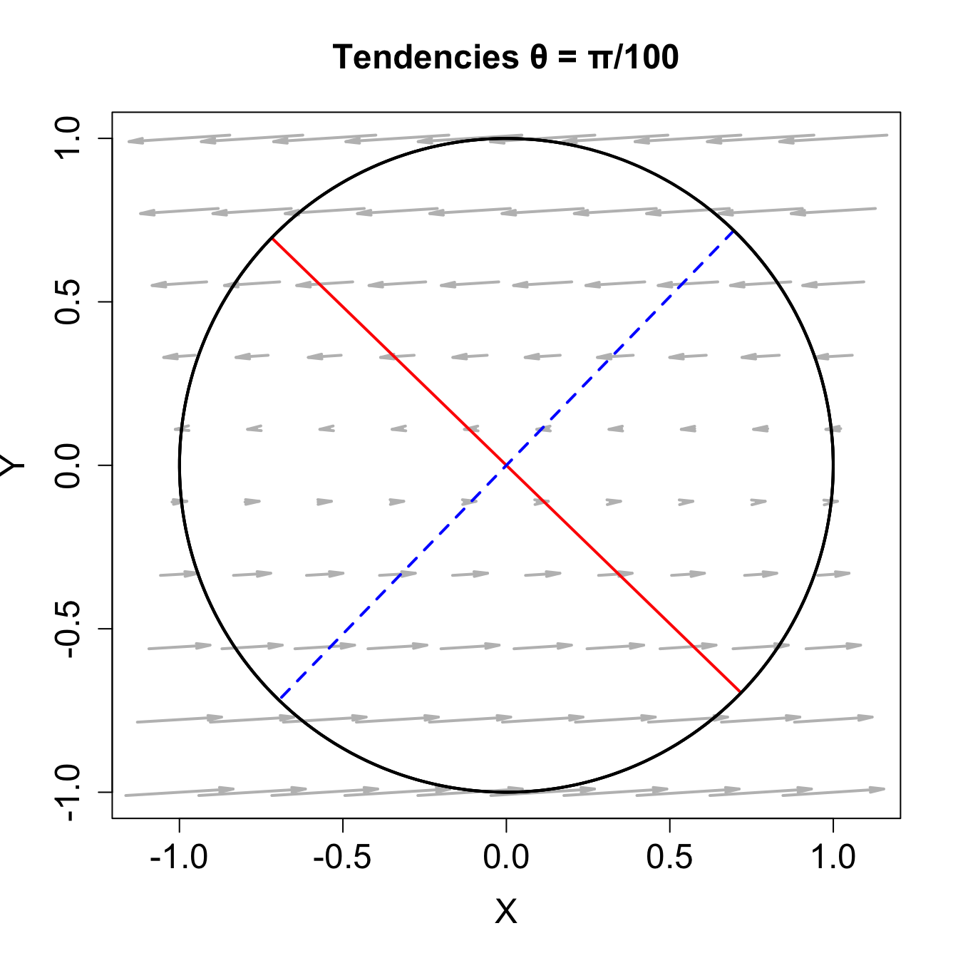
最大瞬時成長率 \(\lim_{t\rightarrow 0}\left\|e^{\mathbf{A}t}\right\|\) は \((\mathbf{A} + \mathbf{A}^\dagger)/2\) の最大固有値で与えられる。 最大瞬時成長は \(\sin\theta < 1/3\) のときに生じる。 最大瞬時成長率を持つ単位ノルム摂動は \(x\) 軸と \(\theta_\alpha = \arctan [(\sin\theta - 1) / \cos\theta]\) の角度をなす。 \(\theta = \pi / 2\) のとき、系は正規となり、数値的最大実部は最も減衰の小さい固有ベクトルの方向である \(x\) 軸と一致し、なす角度は \(\theta_\alpha = 0\) となる。 \(\theta\rightarrow 0\) の極限で非正規性が最大となるが、そのとき \(\theta_\alpha = -\pi/4\) である。
Figure 5.1 に \(\theta = \pi / 100\) のときの時間変化傾向と最大成長及び最大減衰の方向を示す。
Code
<- seq (- 1 , 1 , length.out = 10 )<- seq (- 1 , 1 , length.out = 10 )<- pi / 100 <- atan ((sin (theta) - 1 ) / cos (theta))<- function (theta) {cos (theta) / sin (theta)<- matrix (c (- 1 , 0 , - cot (theta), - 2 ), nrow = 2 )<- expand.grid (x = x, y = y)<- xy$ x<- xy$ y<- amat %*% t (as.matrix (xy))<- 0.005 <- a * uv[1 , ]<- a * uv[2 , ]plot (NULL , xlim = c (- 1 , 1 ), ylim = c (- 1 , 1 ), asp = 1 ,main = expression (paste ("Tendencies " , theta, " = " , pi, "/100" )),xlab = "X" , ylab = "Y" ,cex.main = 1.5 , cex.lab = 1.5 , cex.axis = 1.5 )arrows (X - u, Y - v, X + u, Y + v,col = "gray" , lwd = 2 , length = 0.1 , angle = 10 )segments (cos (alpha), sin (alpha), cos (alpha + pi), sin (alpha + pi), col = "red" , lwd = 2 )segments (cos (alpha + pi/ 2 ), sin (alpha + pi/ 2 ), cos (alpha + 3 * pi/ 2 ), sin (alpha + 3 * pi/ 2 ), col = "blue" , lwd = 2 , lty = 2 )<- pi * seq (0 , 2 * pi, length.out = 361 )lines (cos (angle), sin (angle), col = "black" , lwd = 2 )
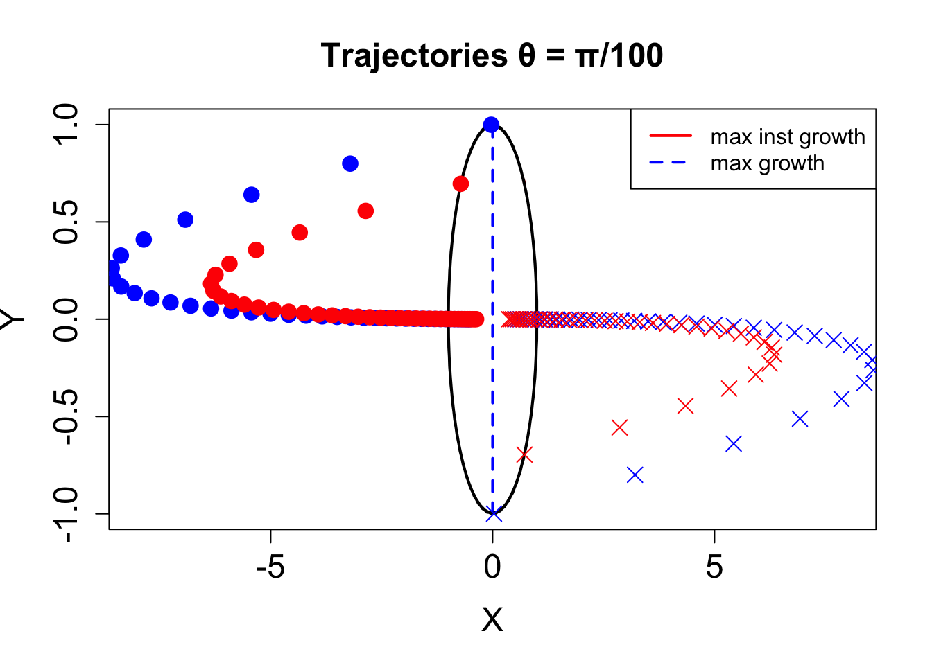
最大瞬時成長及び最大成長を示す摂動の単位円の両端からの時間発展を Figure 5.2 に示す。 減衰が始まるまで、一定時間成長していることが分かる。 大域最適な最大成長は最大瞬時成長よりも、成長が大きい。 最大成長は最も減衰の小さい固有ベクトルの双直交で \((\sin\theta, -\cos\theta)\) 方向に沿っている。
Code
<- 40 <- 0.1 <- function (x, y, dt, nt) {<- rep (0 , nt)<- rep (0 , nt)1 ] <- x1 ] <- yfor (i in 2 : nt) {<- amat %*% c (xhist[i-1 ], yhist[i-1 ])<- xhist[i-1 ] + dt * tendency[1 ]<- yhist[i-1 ] + dt * tendency[2 ] list (x = xhist, y = yhist)plot (NULL , xlim = c (- 8 , 8 ), ylim = c (- 1 , 1 ),# asp = 1, main = expression (paste ("Trajectories " , theta, " = " , pi, "/100" )),xlab = "X" , ylab = "Y" ,cex.main = 1.5 , cex.lab = 1.5 , cex.axis = 1.5 )<- pi * seq (0 , 2 * pi, length.out = 100 )segments (cos (pi/ 2 + alpha), sin (pi/ 2 + alpha), cos (- alpha), sin (- alpha), col = "red" , lwd = 2 )segments (0 , - 1 , 0 , 1 , col = "blue" , lwd = 2 , lty = 2 )lines (cos (angle), sin (angle), col = "black" , lwd = 2 )<- c (sin (theta), sin (theta + pi), cos (alpha), cos (alpha + pi))<- c (- cos (theta), - cos (theta + pi), sin (alpha), sin (alpha + pi))<- c ("blue" , "blue" , "red" , "red" )<- c (4 , 19 , 4 , 19 )for (i in 1 : length (x1)){<- forward (x1[i], y1[i], dt, nt)points (hist$ x, hist$ y, pch = pc[i], cex = 1.5 , col = co[i]) legend ("topright" , c ("max inst growth" , "max growth" ), lw = 2 ,lty = c (1 , 2 ), col = c ("red" , "blue" ))
時刻 \(t\) における時間発展演算子は次のように書ける。
\[
e^{\mathbf{A}t} = \begin{pmatrix}
e^{-t} & \cot\theta(e^{-2t} - e^{-t}) \\
0 & e^{-2t}
\end{pmatrix}
\] \(t\rightarrow\infty\) では
\[
\lim_{t\rightarrow t} e^{\mathbf{A}t} \approx \begin{pmatrix}
e^{-t} & -\cot\theta e^{-t} \\
0 & 0
\end{pmatrix}
\] となるので、
\[
e^{\mathbf{A}t}\begin{pmatrix}\sin\theta\\-\cos\theta\end{pmatrix} =
\frac{e^{-t}}{\sin\theta}\begin{pmatrix}1\\0\end{pmatrix}
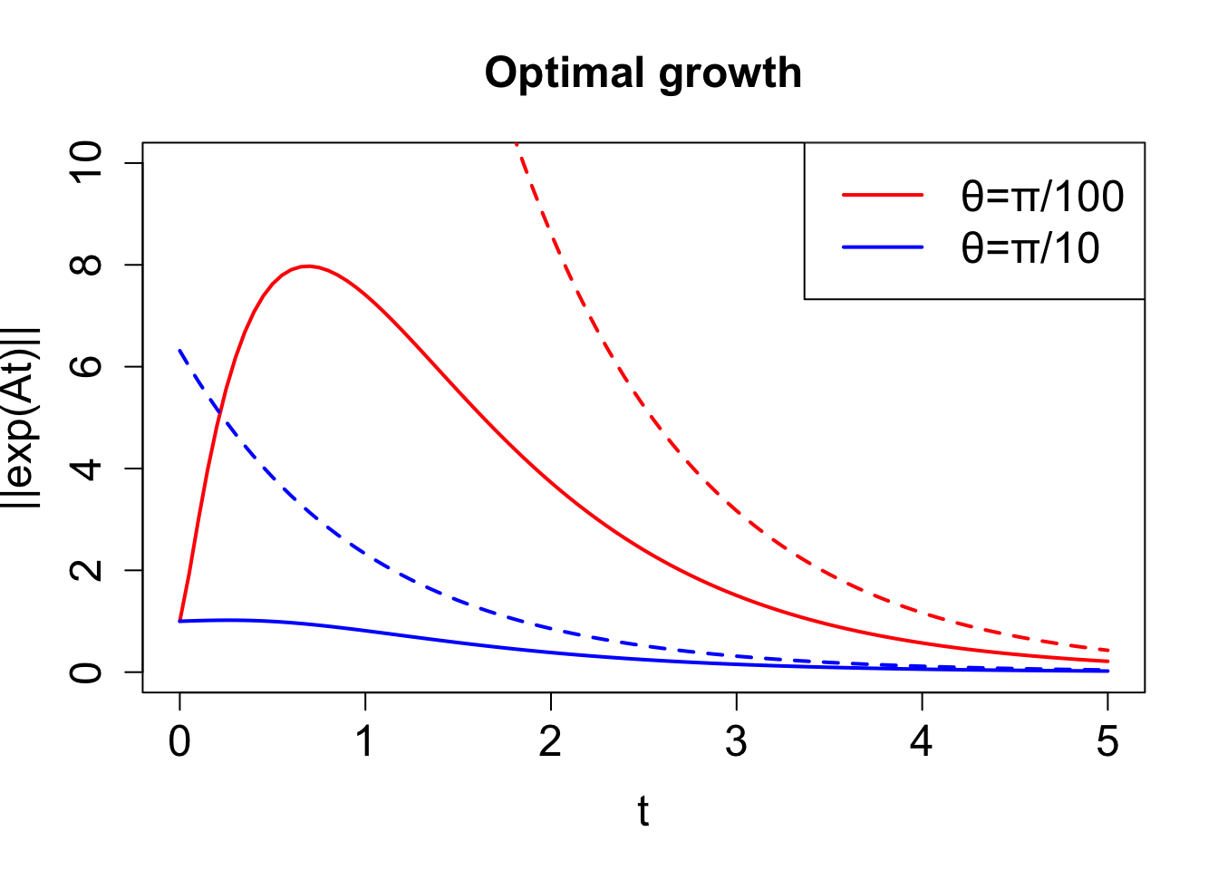
\] となる。 このモードの最適励起がその双直交により生じ、大きさが \(1/\sin\theta\) 倍になることが確認できる。
\(\theta = \pi/100\) 及び\(\theta = \pi/10\) について、最適成長を時間の函数として Figure 5.3 に示す。 成長の上限は演算子の固有ベクトル行列の条件数 \(\kappa(\mathbf{E})=\|\mathbf{E}\|\|\mathbf{E}\|^{-1}\) から Equation 5.4 を考慮して
\[
\left\|e^{\mathbf{A}t}\right\|\le \kappa(\mathbf{E})\left\|e^{\Lambda t}\right\| = \cot\left(\frac{\theta}{2}\right)e^{\lambda_{\max}t}
\tag{5.8}\]
Code
library ("Matrix" )<- function (t, theta) {<- matrix (c (- 1 , 0 , - cot (theta), - 2 ), nrow = 2 )sqrt (max (eigen (expm (t (amat) * t) %*% expm (amat * t))$ values))= - 1 <- seq (0 , 5 , length.out = 101 )<- sapply (ti, optimal.growth, theta)plot (ti, gr, type = "l" , ylim = c (0 , 10 ), lwd = 2 , col = "red" ,cex.main = 1.5 , cex.lab = 1.5 , cex.axis = 1.5 ,main = "Optimal growth" , xlab = "t" , ylab = "||exp(At)||" )lines (ti, cot (0.5 * theta) * exp (lambda.max * ti), lwd = 2 , col = "red" , lty = 2 )<- sapply (ti, optimal.growth, theta * 10 ) lines (ti, gr, lwd = 2 , col = "blue" )lines (ti, cot (0.5 * theta * 10 ) * exp (lambda.max * ti), lwd = 2 , col = "blue" , lty = 2 )legend ("topright" , c (expression (paste (theta, "=" , pi, "/100" )),expression (paste (theta, "=" , pi, "/10" ))), lwd = 2 , col = c ("red" , "blue" ), cex = 1.5 )
Farrell, B. F., and P. J. Ioannou, 1996: Generalized stability theory.
Part I :
Autonomous operators.
J. Atmos. Sci. ,
53 , 2025–2040,
https://doi.org/10.1175/1520-0469(1996)053<2025:GSTPIA>2.0.CO;2 .
Rayleigh, L., 1880: On the resultant of a large number of vibrations of the same pitch and of arbitrary phase.
The London, Edinburgh, and Dublin Philosophical Magazine and Journal of Science ,
10 , 73–78,
https://doi.org/10.1080/14786448008626893 .